Inductively Shunted Superconducting Circuits

In this notebook, we try to reproduce the result of the “Quantization of inductively shunted superconducting circuits” paper.

Introduction

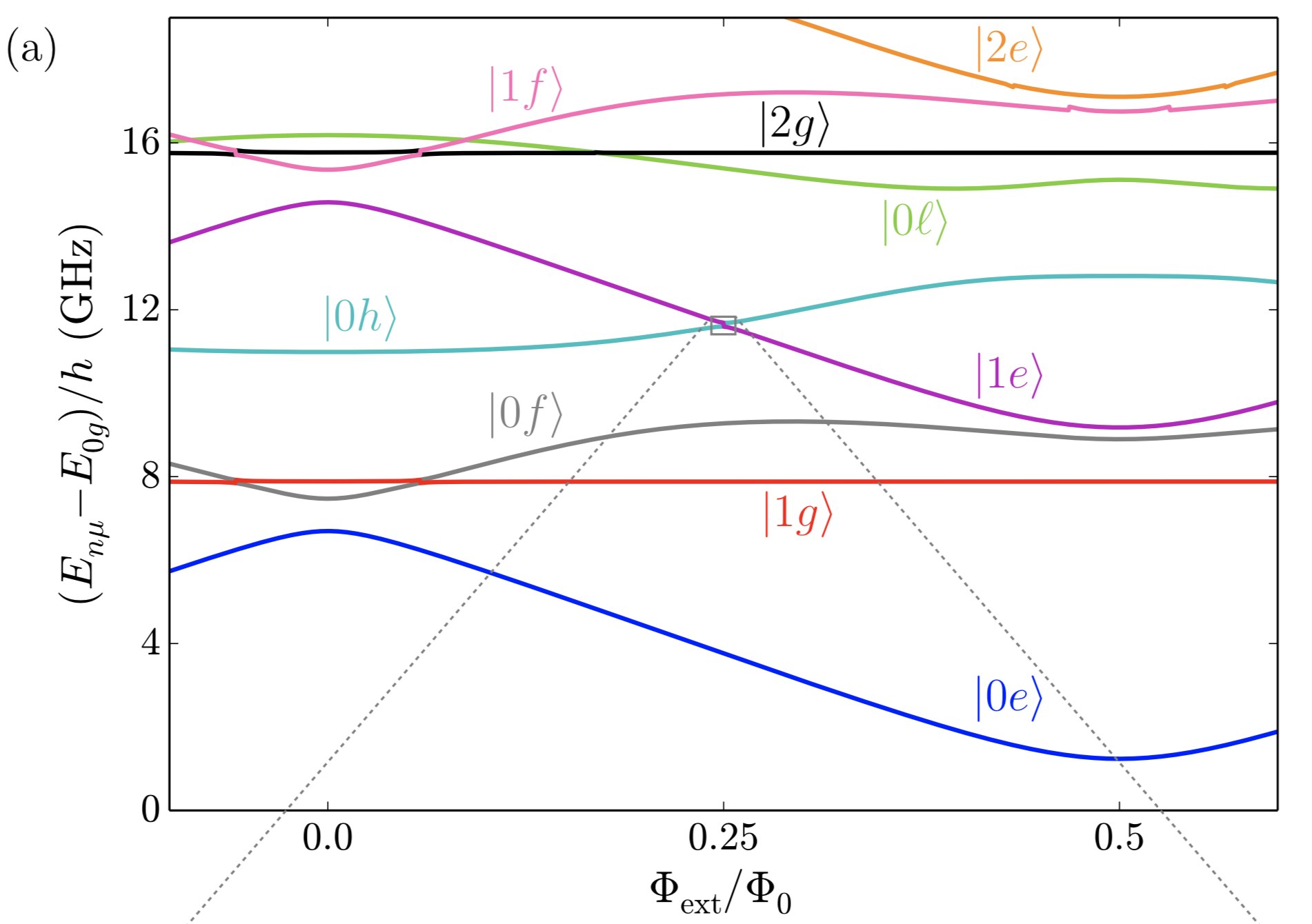
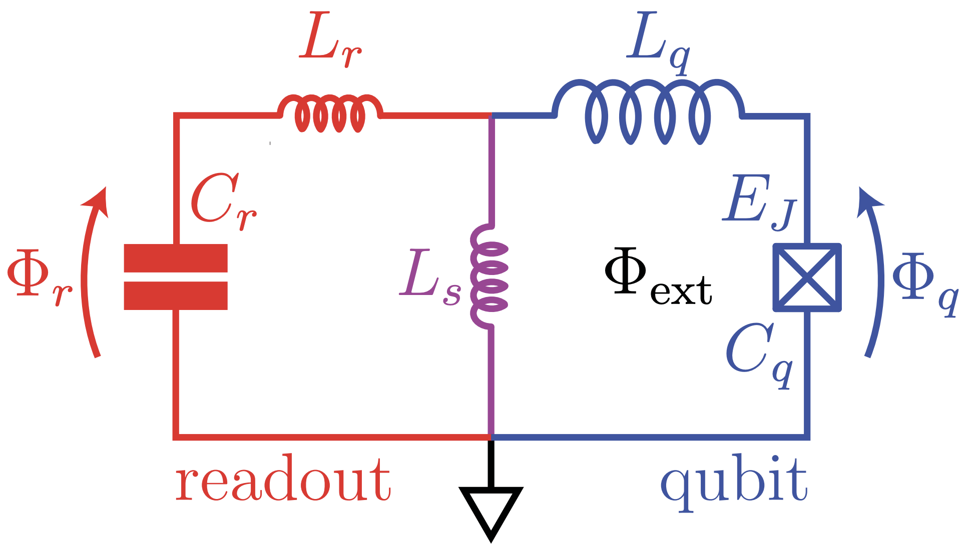
Smith2016 explained how the conventional method or perturbation theory does not correctly diagonalize their highly anharmonic inductively-shunted qubits. However, by using SQcircuit, we simply reproduced the energy spectrum. The diagram of the circuit is

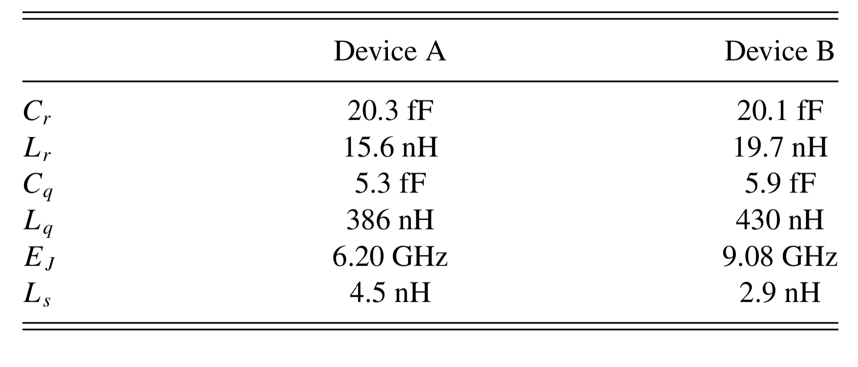
We choose the device A circuit parameters from the following table of the paper:

Circuit Description

Firstly, we import the SQcircuit and the relavant libraries

import SQcircuit as sq
import matplotlib.pyplot as plt
import numpy as np

We define the single inductive loop of the circuit via Loop class

loop1 = sq.Loop()

The elements of the circuit can be defined via Capacitor, Inductor, and Junction classes in SQcircuit, and to define the circuit, we use the Circuit class.

# define the circuit ’s elements
C_r = sq.Capacitor(20.3, "fF")
C_q =  sq.Capacitor(5.3, "fF")
L_r = sq.Inductor (15.6, "nH")
L_q = sq.Inductor(386, "nH", loops=[loop1])
L_s =  sq.Inductor(4.5, "nH", loops=[loop1])
JJ = sq.Junction(6.2, "GHz", loops=[loop1])

# define the circuit
elemetns = {(0, 1): [C_r],
            (1, 2): [L_r],
            (0, 2): [L_s],
            (2, 3): [L_q],
            (0, 3): [JJ,C_q]}

cr = sq.Circuit(elemetns)

By creating an object of Circuit class, SQcircuit systematically finds the correct set of transformations and basis to make the circuit ready to be diagonalized.

Before setting the truncation numbers for each mode and diagonalizing the Hamiltonian, we can gain more insight into our circuit by calling the description() method. This prints out the Hamiltonian and a listing of the modes, whether they are harmonic or charge modes, and the frequency for each harmonic in GHz (the default unit).

cr.description()

$\hat{H} =~\omega_1\hat a^\dagger_1\hat a_1~+~\omega_2\hat a^\dagger_2\hat a_2~+~\omega_3\hat a^\dagger_3\hat a_3~~-~E_{J_{1}}\cos(\hat{\varphi}_1+\hat{\varphi}_2+\hat{\varphi}_3-\varphi_{\text{ext}_{1}})$

$------------------------------------------------------------$

$\text{mode}~1:~~~~~~~~~~~\text{harmonic}~~~~~~~~~~~\hat{\varphi}_1~=~\varphi_{zp_{1}}(\hat a_1+\hat a^\dagger_1)~~~~~~~~~~~\omega_1/2\pi~=~15618.70522~~~~~~~~~~~\varphi_{zp_{1}}~=~2.36e-05$

$\text{mode}~2:~~~~~~~~~~~\text{harmonic}~~~~~~~~~~~\hat{\varphi}_2~=~\varphi_{zp_{2}}(\hat a_2+\hat a^\dagger_2)~~~~~~~~~~~\omega_2/2\pi~=~7.89173~~~~~~~~~~~\varphi_{zp_{2}}~=~3.82e-02$

$\text{mode}~3:~~~~~~~~~~~\text{harmonic}~~~~~~~~~~~\hat{\varphi}_3~=~\varphi_{zp_{3}}(\hat a_3+\hat a^\dagger_3)~~~~~~~~~~~\omega_3/2\pi~=~3.4973~~~~~~~~~~~\varphi_{zp_{3}}~=~2.04e+00$

$------------------------------------------------------------$

$\text{parameters}:~~~~~~~~~~~E_{J_{1}}~=~6.2~~~~~~~~~~~$

$\text{loops}:~~~~~~~~~~~~~~~~~~~~\varphi_{\text{ext}_{1}}/2\pi~=~0.0~~~~~~~~~~~$

The output of description() method specifies that our circuit is consist of three harmonic modes. However, the frequency of the first mode is about 16 THz which is extermly high. Since it is a fast-rotating mode and does not have an impact on the dynamics of the lower eigenvalues of the circuit, we can remove it by setting its truncation number to one.

To determine the size of the Hilbert space, we specify the truncation number for each circuit mode via set_trunc_nums() method. Note that this is a necessary step before diagonalizing the circuit.

cr.set_trunc_nums([1,9,23])

Circuit Spectrum

To generate the spectrum of the circuit, firstly, we need to change and sweep the external flux of loop1 by the set_flux() method. Then, we need to find the eigenfrequencies of the circuit that correspond to that external flux via diag() method. The following lines of code find the spec a 2D NumPy array so that each column of it contains the eigenfrequencies with respect to its external flux.

# number of eigenvalues we aim for
n_eig=10

# array that contains the spectrum
phi = np.linspace(-0.1,0.6,100)

# array that contains the spectrum
spec = np.zeros((n_eig, len(phi)))

for i in range(len(phi)):
    # set the value of the flux external flux
    loop1.set_flux(phi[i])

    # diagonlize the circuit
    spec[:, i], _ = cr.diag(n_eig)

Here we plot the spectrum as a function of external fluxes

for i in range(1,n_eig):
    plt.plot(phi, spec[i,:]- spec[0,:])

plt.xlabel("$\Phi_{ext}/\Phi_0$", fontsize=13)
plt.ylabel(r"$f_i-f_0$[GHz]", fontsize=13)
plt.ylim([0,18])
plt.show()

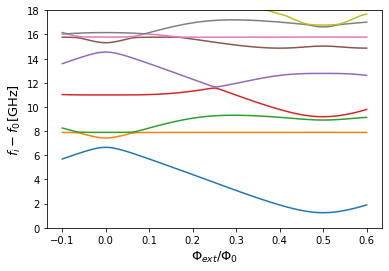
The next cell shows the spectrum from the figure 2 of the paper, which is the same spectrum that SQcircuit calculated.